Disabled Workers and the Indexing of Social Security Benefits
Social Security Bulletin, Vol. 67, No. 4, 2007
This article presents the distributional effects of changing the Social Security indexing scheme, with an emphasis on the effects upon disabled-worker beneficiaries. Although a class of reform proposals that would slow the rate of growth of initial benefit levels over time-including price indexing and longevity indexing-initially appear to affect all beneficiaries proportionally, there can be different impacts on different groups of beneficiaries. The impacts between and within groups are mitigated by (1) the offsetting effect of changes in Supplemental Security Income benefits at the lower tail of the income distribution, and (2) the dampening effect of other family income at the upper tail of the income distribution. The authors present estimates of the size of these effects.
The authors are with the Division of Policy Evaluation, Office of Research, Evaluation, and Statistics, Office of Retirement and Disability Policy, Social Security Administration.
Acknowledgments: The authors wish to thank Richard Balkus, Andrew Biggs, Edward DeMarco, Mike Leonesio, Scott Muller, and Bernard Wixon for particularly helpful comments.
The findings and conclusions presented in the Bulletin are those of the authors and do not necessarily represent the views of the Social Security Administration.
Summary
We examine how benefit amounts and family income would change in response to changing the Social Security (Old-Age, Survivors, and Disability Insurance, OASDI) benefit indexing scheme. We are interested in a class of reform options designed to gradually slow the growth of benefits across the board. These options include the "price indexing" and "longevity indexing" proposals that have been part of the recent Social Security reform debate in the United States as well as a range of proposals developed in Europe.
In this article, we focus on the distributional effects on the disabled. This focus leads to two comparisons. First, we compare disabled-worker beneficiaries to another group that would be affected by the changes, retired-worker beneficiaries. Second, we examine relative changes for particularly vulnerable subgroups of disabled workers.
In the empirical analysis, we use two illustrative examples of potential indexing changes:
- Shifting from wage indexing to price indexing of the initial level of OASDI benefits; and
- Adjusting the initial benefit level for changes in life expectancy at retirement, that is, longevity indexing.
We employ a historical counterfactual simulation to evaluate outcomes that would have resulted from changing the indexing scheme at one particular point in time. The hypothetical implementation period begins with the historical start of the current regime of indexing in 1979 and ends with one of the reference periods of the 1996 Survey of Income and Program Participation (SIPP), a 17-year period. However, we briefly assess the extent to which the results would be applicable to other time horizons.
The analysis uses a cross-sectional sample of OASDI beneficiaries from the 1996 SIPP matched to Social Security administrative records. Further, we use total income from the SIPP (as adjusted to correspond to the calculated OASDI benefit amounts) to simulate eligibility for Supplemental Security Income (SSI) and SSI benefit amounts.
Our overall findings pertain to three outcomes: (1) effects on OASDI benefits viewed in isolation, (2) the offsetting role of SSI, and (3) the diluting effect of other sources of family income. We find that a broader perspective incorporating all three measures is necessary to obtain an appropriate picture of distributional outcomes.
Even though the proposals were designed to have proportional effects, differences between groups—such as disabled and retired workers—can arise from differences in the timing of benefit claiming, mortality, and other factors. Specifically, our cross-sectional estimates suggest that the average change in OASDI benefit levels would be higher for disabled-worker beneficiaries than for retired-worker beneficiaries. These differences are attributable to the fact that a higher proportion of the stock of disabled beneficiaries have been on the Disability Insurance (DI) program rolls for a relatively short period of time and therefore have been affected by the shift in indexing scheme for a longer period of time.
These results must be interpreted within the context of the methodology that was used. Further, other methodologies may lead to different results. For example, in previous studies that restricted the sample to a particular birth cohort, a higher proportion of disabled workers than retired workers were observed to have been on the DI program rolls for a relatively long period of time. Longer time on the beneficiary rolls corresponds to less exposure to the new indexing scheme and smaller estimated benefit changes. Thus, the same underlying factor—the timing of benefit claiming—influences both results.
When the offsetting role of SSI benefits is also considered, we estimate smaller overall changes, especially for those at the bottom of the income distribution. When OASDI and SSI are considered together, differences in average benefit changes between disabled and retired workers are removed. This is due to a higher rate of SSI program participation among disabled workers than among retired workers. In addition, including SSI substantially reduces the proportion of disabled workers that have large simulated changes in benefit amounts.
The estimated effects of changing the indexing scheme are further muted when total family income is considered. This occurs on a roughly equivalent scale for disabled and retired workers. As a result, changing the indexing scheme would produce little change in the status quo differences in poverty status between disabled and retired workers.
Finally, we examine the most economically vulnerable subgroups of OASDI beneficiaries. Within the general group of beneficiaries, we find that the most vulnerable would be less affected than average, primarily as a result of the mitigating effect of SSI benefits. Further, within the population of disabled-worker beneficiaries, we examine economically vulnerable subgroups including those in the lowest primary insurance amount quartile, with less than a high school education, with an early onset of disability, or a primary mental impairment. These groups would also be less affected than average.
Introduction
Various strategies address how to adjust program benefits to protect solvency or contain costs. One class of strategies uses demographic or economic rates of change as a basis for indexing adjustments. For example, Germany uses the ratio of beneficiaries to workers (the dependency ratio) as an input in its retirement system. Also, Sweden partly indexes benefit growth by a measure of the fiscal balance of the retirement system. These indexing approaches are designed to maintain system solvency or sustainability.
The proposals that have been prominent in the recent Social Security reform debate in the United States have proposed indexing adjustments while using different demographic or economic trends as a basis. Some prominent proposals incorporate "price indexing." A common method of implementing price indexing would adjust one part of the benefit formulas that converts past earnings into potential benefit amounts by the difference between wages and prices in successive years. Under this method of implementing price indexing, the initial benefit levels would gradually diverge from the levels dictated by current law; however, benefits would remain constant when viewed through the lens of an alternative theoretical standard. In this case, the alternative standard is a consistent level of purchasing power.
Other proposals incorporate "longevity indexing." Similar to price indexing and other alternatives, longevity indexing would adjust the growth of initial benefits. In this case, the adjustment is according to changes in life expectancy at retirement. Also similar to price indexing, the adjustment maintains benefit levels by an alternative standard, in this case, constant total real lifetime benefits.
The common elements of these indexing approaches are:
- They would slow the rate of growth of benefits while offering an alternative theoretical benefit standard (such as constant purchasing power, constant lifetime total benefits, or some other standard related to system solvency); and
- They could be implemented by gradually adjusting the benefit formulas by changes in an economic or demographic index.
We explore this general class of reform options. Because credible estimates of the effects of the most prominent variants of this class of reform options on the long-term trust fund balances are available (Goss and Wade 2002), we focus on a less explored area—the changing distribution of the well-being of Social Security beneficiaries under alternative indexing schemes. Specifically, we focus on the well-being of disabled-worker beneficiaries under this class of reform options.
At first glance, the distributional effects might appear to be minimal because the same indexing adjustments apply to all new benefit awardees. In fact, a General Accountability Office (GAO 2006) report estimates that there would be a proportional effect on all Old-Age, Survivors, and Disability Insurance (OASDI) beneficiaries. However, we show that there can be differential impacts across groups because of group differences in the timing of benefit claiming, mortality, and other factors. Further, group differences in Supplemental Security Income (SSI) eligibility and participation can lead to differential impacts. Finally, the impact of changes in OASDI benefits on family financial well-being are mitigated by the existing distribution of family income.
We estimate the distributional impact of this class of reform proposals by employing an illustration—based on the counterfactual scenario in which an alternative indexing scheme had been in place between the historical start of the current regime of indexing in 1979 and the national population as sampled in the 1996 SIPP. We illustrate the effects of the two most prominent proposals, price indexing and longevity indexing. Because the two proposals would be implemented using the common mechanism, the illustrations produce similar distributional results.
The rest of this article is organized as follows. We begin by describing the class of alternative indexing approaches addressed in our study, which is followed by a contrasting of possible analytical approaches. Next, we discuss the simulation methodology and then proceed to describe baseline differences in the economic well-being of disabled and other beneficiaries. The simulation results of changing the indexing of benefits are presented next and are followed by a discussion, in the conclusions and implications section, of the generalizability of the results.
Indexing Approaches
An individual's basic OASDI benefit level, known as the primary insurance amount (PIA), is a function of lifetime earnings, measured as average indexed monthly earnings (AIME), the PIA bend points, and the PIA factors. There are two PIA bend points, which divide the PIA into three terms, each of which consists of a PIA factor multiplied by the portion of the AIME that falls into the interval defined by the bend points. The three PIA factors are 90 percent, 32 percent, and 15 percent. For example, in 1996, the first PIA bend point was $437 and the applicable PIA factor is 90 percent. The first term would be the lesser of the AIME or $437 multiplied by the factor of 90 percent. The other terms are calculated in a similar manner.
Wage indexing affects benefit levels under current law in two ways. First, the PIA bend points are indexed to wage growth, and second, wage trends are used to inflate earnings in previous years to current levels. In addition, wage indexing affects system revenues through the proportion of earnings that is subject to the payroll tax, known as the taxable maximum. The average wage index enters the benefit and revenue formulas in these three ways.
According to the President's Commission to Strengthen Social Security (CSSS 2001, 120), the policy of switching from wage indexing to price indexing "would be implemented by multiplying the PIA bend point factors (the [PIA] bend points would remain indexed to wages) by the ratio of the Consumer Price Index to the Average Wage Index in successive years."1 The three ways in which wage indexing enters the current law formulas would remain intact and the PIA factors, which are not currently indexed, would be modified by the CSSS method.
This is not the only possible method of implementation. For example, Biggs, Brown, and Springstead (2005) explore the properties of replacing the parts of the benefit formulas that are currently wage indexed with price indexing. They consider the variants of price indexing the AIME, price indexing the PIA bend points, and the combination of price indexing the AIME and the PIA bend points (in addition to considering the CSSS method).2 The CSSS method, applying price indexing to the PIA factors, is the most widely accepted method,3 however, and is used by the Social Security Administration's Office of the Chief Actuary in its evaluations (see Chaplain and Wade (2005) and Goss and Wade (2002) for example).
The CSSS method proposes to multiply each term by a constant that is unique to each annual awardee cohort. The constant can be factored out; thus, the method is equivalent to multiplying the initial benefit level by a constant that is unique to each year. The constant is the ratio of price growth to wage growth between the start of the indexing regime and the start of benefit receipt (both with 2-year lags). This method adjusts benefits proportionally for all beneficiaries who begin receiving benefits in a specific year. Other than by year of the start of benefit receipt, the proportional adjustment would not vary across individuals.
In addition to price indexing, the general class of reform proposals can be implemented by adjusting the PIA factors. In this article, we also simulate adjusting for longevity. The adjustments would be based on changes in life expectancy conditional on having reached retirement age.4 The CSSS recommends basing these adjustments on changes over 10-year periods with subsequent reevaluations every 10 years.5
Several features of this indexing approach are notable. For individuals retiring in successive years with similar retirement benefit levels, this adjustment keeps the expected total sum of real benefit payments roughly constant.6 Also, the adjustment for life expectancy reflects changes in average life expectancy for a cohort at a particular point in the life cycle rather than for individuals or particular demographic groups. For example, markedly different life expectancies apply to people with disabilities and there is further variation by diagnosis (Rupp and Scott 1998). If the adjustment for life expectancy of the population at retirement age were applied to all new awardees, then other groups of beneficiaries, such as disabled-worker beneficiaries, would be affected as well.
The analysis is based on the assumption that changes in OASDI indexing formulas for retired-worker awardees would apply equivalently to disabled-worker awardees. Following the CSSS,7 this should not be interpreted as a policy recommendation but rather as an illustration of the effect that the proposed indexing approaches would have on disabled-worker beneficiaries. In fact, some recent policy proposals exempt disabled workers from indexing changes (see Goss and Wade (2006) for example), and the Government Accountability Office (2007) discusses the methods by which this could be implemented.
Analytical Approaches
There are different perspectives from which to view the impact of changes in the Social Security indexing scheme. First, one can estimate the effect on a cohort of benefit awardees, which allows for comparing, for example, subgroups of a given awardee cohort after implementation of a new indexing scheme. Second, one can analyze the effect on a birth cohort as it progresses through the life cycle, which allows for comparing outcomes for subgroups of the same birth cohort. Third, one can analyze a cross section of the beneficiary population at a given point in time, which allows for examination of the effects on different subgroups of current beneficiaries, such as subgroups defined by marital status, poverty status, or type of OASDI beneficiary. The different perspectives seek answers to different questions, a fact that is important to keep in mind when interpreting results. Some of the results may differ based on the analytic perspective used, while others may be robust across different perspectives.
When analyzing changes in the Social Security indexing scheme, a beneficiary awardee cohort approach is sometimes implied. In an example of this analytical approach, GAO (2006, 4) states:
Regardless of the index, adjusting the initial benefit level through the benefit formula typically would have a proportional effect, with constant percentage changes at all earnings levels, on the distribution of benefits.
As will be explained below, differences in the impact of indexing changes can arise from differences in the timing of benefit claiming. Thus, statements such as the one above assume that there are no differences in the timing of benefit claiming and apply to groups that are similar in this regard, that is, people in the same benefit awardee cohort.
By contrast, differences in the timing of benefit claiming arise when viewing the impacts from a birth cohort perspective. For example, Mermin (2005, 7) predicts that:
Because the effect of substituting price indexing for wage indexing is cumulative over time, individuals who become eligible for benefits earlier experience relatively smaller reductions compared with scheduled amounts. Disability recipients and survivors often become eligible for benefits before age 62 and therefore receive smaller reductions in initial benefits under price indexing.
The difference in group impacts between disabled and retired workers is a direct result of choosing a birth cohort analytical perspective.8 From this perspective, disabled workers appear less vulnerable to changes in the indexing scheme than do retired workers.
Different outcomes might be expected from a cross-sectional analytical perspective, at least when OASDI benefit changes are analyzed in isolation. A cross-sectional analysis examines a stock of beneficiaries at a specific point in time after the simulated start of the new indexing scheme. By construction, benefit changes for each beneficiary will be a function of the time between the simulated start of the new indexing scheme and the cross-sectional observation point as well as observed duration on the program rolls at that point. The first of these factors is constant across individuals at the time, while duration may vary. Since the duration of the period in beneficiary status is inversely related to the period subject to the new indexing scheme, it will also be inversely related to the size of the impact of the change in indexing scheme. If disabled workers have a shorter average duration than retired workers, one might expect relatively large percent changes in OASDI benefits for the disabled. As was the case with the birth cohort analytical perspective, this result is strongly influenced by the choice of a cross-sectional analytical perspective.
Methodology
We employ a cross-sectional sample from the 1996 Survey of Income and Program Participation (SIPP). Our study universe is all noninsitutionalized adults (aged 18 or older) in current OASDI pay status in November 1996. The sample is extracted from wave 3 of the 1996 SIPP. Observations without a match to the Summary Earnings Record (SER)—14.8 percent—are excluded and the sampling weights are adjusted accordingly. Participation in the Disability Insurance (DI) and SSI programs is defined as having a positive benefit indicated in the Master Beneficiary Record and Supplemental Security Record, respectively.
We estimate the effects of two indexing approaches that employ price indexing or life expectancy indexing in the determination of the initial level of benefits. We present estimates of the effect on the current stock of OASDI beneficiaries. This represents the "direct effect" (Bound and others 2002) of the indexing schemes. Estimates of "indirect effects" are left for future research; we assume that the indexing approaches do not lead to changes in participation in the OASDI and SSI programs. Changes in benefit amounts for current participants are estimated for both programs.
We construct a benefit calculator that estimates AIME and insured status based on the earnings history recorded in the SER. The PIA is obtained by applying the benefit formula to the AIME. We calculate OASDI benefit amounts for the individual and spouse but not other family members.9 Benefit amounts are calculated at the initial entitlement date and updated using price indexing.10, 11 The PIA factors are then multiplied by the relevant ratio in order to implement the two indexing approaches.
The indexing approaches are implemented by applying the long-term trend in both real wages and life expectancy. In the half century from 1951 to 2002, wages increased by 4.97 percent per year compared with only 3.81 percent per year for prices. The difference of 1.16 percentage points a year measures the gain in real wages and is used in the formula adjustments. For life expectancy, an increase of one-half of one percent per year is used, as recommended by the CSSS. This is compatible with the average changes over the 1940 to 2002 period (Bell and Miller 2002).12
We apply the adjustments to observations that have an initial entitlement date after the historical start of the current regime of indexing, 1979.13 Over the 17-year period from this date to the reference period of the sample (November 1996), the maximum change in benefits based on changes in real wages is less than 18 percent. For adjustments based on life expectancy, the maximum change is slightly more than 8 percent.
Benefit amounts are tied to the earnings record of the spouse in many cases, so we also consider the calculated benefit of living spouses and the relevant program rules, but do not attempt to link to previous or deceased spouses; thus, we do not calculate survivor or other benefits that are not based on the individual's or living spouse's earnings records. Those types of benefits fall under the "other beneficiaries" headings in the tables. In the simulations, we impose the average percentage benefit change for the calculated benefit amounts (by age group) to simulate the change in benefit amounts for these benefit types.
We present simulation results using the individual beneficiary as the unit of observation and calculate OASDI benefits for the reference person and for the individual's "unit." The unit includes the spouse if the individual is married and the spouse is present, otherwise the unit includes only the individual. This construction is similar to the concept used in the SSI program, which determines financial eligibility for individuals or couples.
When simulating financial eligibility for SSI, we evaluate income and resources, and consider spousal deeming rules.14 Countable resources and countable income are measured in the SIPP (see Davies and others (2001/2002) for more information). Because SSI benefit receipt is often misreported in the SIPP (Huynh, Rupp and Sears 2002), we use administrative records to determine program participation. Benefit amounts also may be misreported. Thus, we replace self-reported OASDI and SSI benefit amounts with administrative amounts for the family members for whom we do not calculate benefit amounts (those outside of the unit).15
The Well-Being of the Disabled
We analyze the initial position of the group of disabled-worker beneficiaries from two perspectives. First, we measure the well-being of the group of disabled-worker beneficiaries relative to other groups, and second, we measure the well-being of subgroups of disabled-worker beneficiaries relative to other subgroups. Of the many aspects of well-being, we restrict the analysis to financial well-being and focus on changes in income.
The Relative Well-Being of the Disabled
The population of interest in this article is generally the baseline set of disabled-worker beneficiaries. Comparisons of this group with retired-worker beneficiaries are central to our study, and therefore we assess baseline differences between the two groups. Also, we compare disabled-worker beneficiaries with the group of nonbeneficiaries because this group is a valuable comparison group composed mainly of nondisabled working-aged people. A comparison of the characteristics of disability beneficiaries with these two comparison groups is shown in Table 1.16, 17
| Variable subgroup | OASDI beneficiaries | Non- beneficiaries a |
||
|---|---|---|---|---|
| Disabled workers |
Retired workers |
Other beneficiaries |
||
| Economic variables | ||||
| Total family income (dollars, monthly) | 2,624 (97) |
2,617 (29) |
2,353 (59) |
4,317 (21) |
| Poverty rate (percent) | 24.0 (1.3) |
8.7 (0.3) |
15.0 (0.7) |
12.6 (0.2) |
| Programmatic variables | ||||
| OASDI benefit of individual (dollars) b | 663 (8) |
706 (3) |
601 (7) |
. . . |
| Duration of benefit receipt (years) | 7.2 (0.2) |
11.4 (0.1) |
11.9 (0.2) |
. . . |
| OASDI benefit of unit (dollars) c | 710 (9) |
1,046 (6) |
861 (10) |
. . . |
| SSI financial eligibility (percent) | 20.7 (1.2) |
5.4 (0.3) |
13.8 (0.7) |
10.5 (0.1) |
| SSI participation among eligibles (percent) | 71.9 (2.9) |
50.3 (2.3) |
63.3 (2.6) |
2.0 (0.1) |
| OASDI plus SSI benefit of unit (dollars) | 733 (9.0) |
1,052 (6.0) |
879 (10.0) |
. . . |
| Demographic variables | ||||
| Age (years) | 47.7 (0.3) |
72.4 (0.1) |
67.8 (0.3) |
38.9 (0.1) |
| Women (percent) | 41.7 (1.4) |
47.3 (0.6) |
93.5 (0.5) |
51.2 (0.2) |
| Married (percent) | 47.1 (1.5) |
59.5 (0.6) |
36.5 (1.0) |
58.6 (0.2) |
| Family size | 2.5 (*) |
1.9 (*) |
2.0 (*) |
3.0 (*) |
| Household size | 2.7 (*) |
2.0 (*) |
2.1 (*) |
3.2 (*) |
| Reside in a metropolitan statistical area (percent) | 71.6 (1.3) |
74.0 (0.5) |
69.4 (1.0) |
78.0 (0.2) |
| Black (percent) | 19.4 (1.2) |
8.4 (0.3) |
10.0 (0.6) |
11.4 (0.2) |
| Hispanic (percent) | 5.9 (0.7) |
3.9 (0.2) |
5.3 (0.5) |
9.5 (0.1) |
| Completed high school (percent) | 68.1 (1.4) |
67.2 (0.5) |
57.2 (1.0) |
86.3 (0.2) |
| Health and mortality variables | ||||
| Poor health (percent) | 36.9 (1.4) |
12.2 (0.4) |
13.0 (0.7) |
2.4 (0.1) |
| Nights spent in hospital (annual number) | 4.1 (0.4) |
2.0 (0.1) |
1.7 (0.1) |
0.4 (*) |
| Doctor visits (annual number) | 17.1 (1.0) |
7.4 (0.2) |
7.9 (0.4) |
4.4 (0.1) |
| Any functional impairment (percent) d | 53.6 (1.5) |
26.7 (0.5) |
37.9 (1.0) |
4.7 (0.1) |
| Work limitation in two periods (percent) | 73.1 (1.3) |
5.4 (0.3) |
12.8 (0.7) |
4.3 (0.1) |
| Death within 4 years of survey (percent) | 8.9 (0.8) |
13.7 (0.4) |
11.1 (0.7) |
0.9 (*) |
| Numbers of observations (unweighted) | 1,161 | 7,555 | 2,302 | 42,804 |
| SOURCES: Calculations based on the Survey of Income and Program Participation (SIPP) matched to Social Security administrative records. | ||||
| NOTES: The survey reference month is November 1996. The sample is restricted to adults who have SIPP observations that have been successfully matched to the Summary Earnings Record. Sampling weights have been adjusted by the inverse of the matching rate. Standard error estimates assume simple random sampling and are included in parentheses. | ||||
| . . . = not applicable; * = less than 0.05; OASDI = Old-Age, Survivors, and Disability Insurance; SSI = Supplemental Security Income. | ||||
| a. The sample is restricted to people aged 18 or older. | ||||
| b. Values are for the sample reference person. | ||||
| c. Values are for the sample reference person if unmarried and for the reference person and spouse combined if married (spouse present). | ||||
| d. Including difficulty with any activities of daily living (ADL) or instrumental activities of daily living (IADL). | ||||
DI beneficiaries differ most notably from these two comparison groups in terms of a variety of health measures. For disabled workers, 36.9 percent describe their health status as poor compared with only 2.4 percent in the nonbeneficiary population and 12.2 percent of retired workers. In addition, 53.6 percent of disabled workers report some sort of functional limitation, about twice the percentage of retired workers and more than ten times the percentage in the nonbeneficiary population. These patterns are confirmed by more objective self-reported health measures such as the number of hospital and doctors visits. These differences are all statistically significant.
The demographic composition of the group of disabled workers also differs from the other two groups. Compared with retired workers, disabled workers are of course younger on average but also less often married and more often black. Also, disabled workers live in larger households and families. Compared with the nonbeneficiary population, disabled workers are older, less often female, married, or Hispanic, and more often black. By contrast to the comparison with retired workers, disabled workers live in smaller households and families than the nonbeneficiary population. Also, they are less likely to have completed high school. All of these differences are also statistically significant.
Disabled workers also differ from the two comparison groups in terms of benefit amounts. For average OASDI benefits, the difference between disabled and retired workers is statistically significant, however, the dollar amounts are relatively small. Of course, nonbeneficiaries receive no benefit from OASDI, which is a fundamental difference between them and the beneficiary groups.18
As mentioned, disabled workers are less likely to be married than are members of the comparison groups. Compared with retired workers, this contributes to a lower probability that the disabled worker has a spouse with OASDI benefits. When OASDI benefits are calculated for the individual's unit (including the benefits of a spouse if present), a difference is observed that is both statistically significant and a meaningful dollar amount (more than $300 lower for disabled workers per month).
In contrast to spouse benefits, the receipt of SSI is much more important for disabled workers than for retired workers. As shown in Table 1, 20.7 percent of disabled workers are estimated to be financially eligible for SSI versus only 5.4 percent of retired workers. Further, 71.9 percent of financially eligible disabled workers participate in the SSI program versus only 50.3 percent for retired workers. Thus SSI adds more to the average OASDI benefit for disabled-worker beneficiaries ($23 on the average) than for retired-worker beneficiaries ($6 on the average) on a unit basis.19 Still, the combined OASDI and SSI benefits of the unit are smaller for disabled workers than they are for retired workers mainly because the inclusion of the spouse's OASDI benefit far outweighs the opposing effect of SSI.
In general, total benefits (OASDI and SSI combined) are smaller for disabled workers than retired workers. Further, the differences in the prevalence of low benefits may be larger than suggested by the means. Chart 1 shows the distributions of total benefits for the two groups as bar charts overlaid by kernel density functions.20 For disabled workers, the distribution is skewed such that the most probable benefit amount is smaller than the mean. By contrast, the distribution for retired workers is bimodal because of the role of spouse benefits21 with one peak above and one peak below the mean. Thus, relatively more disabled workers have low levels of benefits than is indicated by relative differences in the means. We will examine some groups of disabled workers that are more likely to appear in the lower tail of the distribution in the next section.
Distribution of total benefits (OASDI and SSI) for disabled- and retired-worker beneficiaries
Text description for Chart 1.
Distribution of total benefits (OASDI and SSI) for disabled- and retired-worker beneficiaries
This chart has two separate panels of bar charts. One panel shows data for disabled-worker beneficiaries and the other shows data for retired-worker beneficiaries.
In both panels, the horizontal axis shows total benefit dollar amounts and the vertical axis shows the percentage of beneficiaries. Vertical bars in each panel indicate the percentage of beneficiaries with benefits at certain dollar amounts.
In the disabled-worker panel, the bars reach the following approximate coordinates: two percent at 160 dollars; five percent at 320 dollars; 33 percent at 480 dollars; 18 percent at 640 dollars; 16 percent at 800 dollars; 10 percent at 960 dollars; nine percent at 1,120 dollars; four percent at 1,280 dollars; one percent each at 1,400, 1,600, and 1,760 dollars; and one-half of one percent at 1,930 dollars.
In the retired-worker panel, the bars reach the following approximate coordinates: two percent at 120 dollars; eight percent at 350 dollars; 17 percent at 570 dollars; 23 percent at 800 dollars; 11 percent at 1,030 dollars; nine percent at both 1,260 and 1,490 dollars; 13 percent at 1,720 dollars; six percent at 1,940 dollars; and one-half of one percent at both 2,170 and 2,400 dollars.
In addition to the bars, a line labeled Kernal density function appears on both panels. The line roughly follows the tops of the vertical bars. For disabled workers, the line is generally slightly above the tops of the bars; for retired workers, it is generally slightly below the tops of the bars.
Measuring overall economic vulnerability involves more than just benefit amounts. It is necessary to consider the individual in the broader context of family consumption and benefit amounts in the broader context of family income to get an accurate picture. Although both disabled and retired workers are in families with significantly lower income than nonbeneficiaries, they do not significantly differ from each other in terms of average family income. This is the net result of two factors that work in opposite directions. The combined OASDI and SSI income of the unit is significantly larger for retired workers as we have seen. However, the families of disabled workers have more income from other sources. The share of other income is 72 percent for disabled workers, while it is only 60 percent for retired workers.22 This is related to the larger family size of disabled workers.
Once we look at distributional indicators that adjust for family size, the substantial differences in the economic well-being of disabled-worker and retired-worker beneficiaries becomes transparent. Disabled worker beneficiaries experience much higher poverty rates than retired workers or nonbeneficiaries (see Table 1), and the differences are statistically significant.
Well-Being within the Group of Disabled Beneficiaries
Disabled workers as a group form an economically vulnerable segment of OASDI beneficiaries. We operationally define beneficiaries as economically vulnerable if their family income is at or below the official poverty threshold. Accordingly, a subgroup of disabled workers is defined as economically vulnerable if the proportion that is classified as poor is high compared with the rate for disabled workers as a whole. We define economically vulnerable subgroups on the basis of four variables commonly believed to be associated with the risk of economic vulnerability. The subgroups of disabled workers include (1) those in the lowest PIA quartile, (2) those with less than a high school education, (3) beneficiaries with an early onset of disabilities, and (4) those with a primary mental impairment. These subgroups display poverty rates ranging from 30 percent to 44 percent (Table A-1)—compared with the average of 24 percent for all disabled beneficiaries.
What is the contribution of various income sources to alleviating economic vulnerability? We distinguish three principal sources of family income: OASDI, SSI, and other income (from any source except OASDI or SSI). We first look at the subgroup directly defined by economic vulnerability: disabled workers in poverty. The first set of bars on Chart 2 presents their average income as a percent of the corresponding average for all disabled workers from each of the three sources. The data show that relatively low income from OASDI and especially from other sources are the reasons for economic vulnerability among poor disabled workers. By contrast, SSI plays a mitigating role.
Average family income by source as a percent of the average for all disabled-worker beneficiaries,
by selected subgroups
| Subgroup | OASDI | SSI | Other |
|---|---|---|---|
| Below poverty line | 67 | 252 | 8 |
| Lowest PIA quartile | 55 | 339 | 89 |
| Less than high school | 93 | 157 | 68 |
| Aged 18–34 at award | 79 | 178 | 91 |
| Mental impairment | 83 | 174 | 83 |
A complementary perspective is provided by the share of income from various sources for disabled workers in poverty. More than two-thirds of their income (69 percent)23 comes from OASDI, and less than a fourth comes from other income sources (besides SSI). This suggests that the effects of any OASDI changes might not be much dampened by the cushion of other family income. Thus, those in poverty are not only the most economically vulnerable under the baseline, but also vulnerable to OASDI changes.
Chart 2 also presents the average income of the four other economically vulnerable subgroups identified above relative to the average for all disabled workers. Not surprisingly, the overall patterns are similar to the findings for disabled workers in poverty. The one difference for all four of these groups is that income from other sources is much closer to the average.
Interestingly, there are other groups of disabled beneficiaries that are often thought of as vulnerable that do not meet the criteria of economic vulnerability we employ here. For example, severity of disabilities is not clearly associated with economic vulnerability (again see Table A-1). Being close to the end of one's life during the reference month (as measured by death within 4 years of the survey) is also not associated with economic vulnerability. The figures for high mortality risk (as measured by death within 4 years of onset of disability) are also at least suggestive of the absence of a positive relationship between high mortality risk and economic vulnerability.24
The Effects of Changing the Indexing of Benefits
In this section we describe the overall results of the two simulations on OASDI benefits, OASDI and SSI combined, family income, and the poverty rate. Next, we identify the general distributional effects underlying the overall patterns of results and, finally, examine changes within the group of disabled-worker beneficiaries.
Group Effects
We analyze both estimated average changes and the variability of those outcomes for both disabled workers and retired workers. Further, we explore the ways in which SSI and other family income mitigate the effects of the indexing approaches. As we shall see, looking at OASDI benefits alone may lead to misleading conclusions; other sources of family income also need to be considered.
OASDI Benefit Changes. The percentage changes in OASDI benefit levels corresponding to the indexing approaches are larger for disabled workers than for retired-worker beneficiaries. The first column of Table 2 presents the average results overall and for relevant subgroups of the OASDI beneficiary population. For both price indexing and life expectancy indexing, disabled workers are more affected than retired workers and the differences are statistically significant.25 As will be explained in the General Distributional Effects subsection, this is related to average differences in the timing of benefit entitlement between retired and disabled workers that is a direct consequence of our choice of a cross-sectional analytical approach.
| Indexing option and OASDI beneficiary subgroup |
Individual OASDI benefits a (percent change) |
Unit OASDI benefits b (percent change) |
Unit OASDI plus SSI benefits b (percent change) |
Family income (percent change) |
Poverty rate (percentage- point change) |
|---|---|---|---|---|---|
| Price indexing | |||||
| All beneficiaries | -9.6 (0.049) |
-9.6 (0.048) |
-9.0 (0.051) |
-4.7 (0.036) |
2.0 (0.134) |
| Disabled worker | -10.6 (0.159) |
-10.7 (0.157) |
-9.1 (0.185) |
-4.4 (0.127) |
2.1 (0.423) |
| Retired worker | -9.1 (0.063) |
-9.2 (0.060) |
-8.9 (0.062) |
-4.6 (0.043) |
1.7 (0.150) |
| Of which: | |||||
| Former disabled worker | -5.3 (0.182) |
-5.7 (0.178) |
-5.3 (0.178) |
-3.2 (0.123) |
1.5 (0.428) |
| Never a disabled worker | -9.5 (0.064) |
-9.6 (0.062) |
-9.4 (0.064) |
-4.8 (0.045) |
1.7 (0.160) |
| Other | -10.7 (0.069) |
-10.0 (0.082) |
-9.1 (0.100) |
-5.0 (0.078) |
3.0 (0.388) |
| Life expectancy indexing | |||||
| All beneficiaries | -4.6 (0.023) |
-4.6 (0.023) |
-4.3 (0.024) |
-2.3 (0.017) |
1.0 (0.095) |
| Disabled worker | -5.0 (0.076) |
-5.1 (0.075) |
-4.3 (0.088) |
-2.1 (0.060) |
1.2 (0.323) |
| Retired worker | -4.3 (0.030) |
-4.4 (0.029) |
-4.3 (0.030) |
-2.2 (0.021) |
0.8 (0.104) |
| Of which: | |||||
| Former disabled worker | -2.5 (0.087) |
-2.7 (0.085) |
-2.5 (0.085) |
-1.5 (0.059) |
0.9 (0.330) |
| Never a disabled worker | -4.5 (0.031) |
-4.6 (0.030) |
-4.5 (0.031) |
-2.3 (0.022) |
0.8 (0.110) |
| Other | -5.1 (0.033) |
-4.8 (0.039) |
-4.3 (0.048) |
-2.4 (0.037) |
1.6 (0.284) |
| SOURCES: Calculations based on the Survey of Income and Program Participation (SIPP) matched to Social Security administrative records. | |||||
| NOTES: The survey reference month is November 1996. The sample is restricted to adults who have SIPP observations that have been successfully matched to the Summary Earnings Record. Sampling weights have been adjusted by the inverse of the matching rate. Standard error estimates assume simple random sampling and are included in parentheses. | |||||
| OASDI = Old-Age, Survivors, and Disability Insurance; SSI = Supplemental Security Income. | |||||
| a. Values are for the sample reference person. | |||||
| b. Values are for the sample reference person if unmarried and for the reference person and spouse combined if married (spouse present). | |||||
When the OASDI benefit of the spouse, if any, is considered in combination with the beneficiary (second column), the results are similar. Although the OASDI benefit of the spouse can potentially have a large effect on the level of total benefits in the base case, the percentage changes in outcomes are robust with respect to the inclusion of the benefit of the spouse. This implies that the effect of changing the indexing approach on the benefit of the spouse is equivalent to the effect on the individual's benefit, on average.26, 27
Although the comparison of averages is a useful first step, the variability of the estimated changes also needs to be considered. Even if the magnitude of average changes is somewhat larger for the disabled, it is possible that a substantially smaller portion of disabled workers would experience large changes compared with retired workers and, thus, the consideration of distributional detail would make the results more ambiguous. However, we find that a substantially larger portion of disabled workers are expected to experience relatively large OASDI changes. This can be seen in the top panel of Chart 3. This chart summarizes the distributions for disabled- and retired-worker beneficiaries of OASDI benefit changes (top panel) and changes in OASDI and SSI benefits combined (bottom panel) for the price indexing simulation.28 Looking at the top panel we see that the distribution of OASDI changes for the disabled is bimodal, with a large peak at the high end of the estimated changes (on the left), and a smaller peak at the low end of the distribution (on the right). By contrast, the peak indicating large changes (on the left) is much smaller for retired workers. The peak indicating relatively small changes (on the right) is relatively close for the two groups. Importantly, there is a third peak for retired workers that is the highest (in the middle) and centers around the average. Thus, a substantially higher portion of disabled workers are estimated to experience relatively large OASDI benefit changes under price indexing. This also holds for life expectancy indexing, as seen in Chart A-1. The shape of the distribution of changes corresponding to the two indexing schemes is very similar.
Distribution of simulated changes in benefits under price indexing for disabled- and retired-worker beneficiaries
Text description for Chart 3.
Distribution of simulated changes in benefits under price indexing for disabled- and retired-worker beneficiaries
This chart shows four separate panels of bar charts. The first two panels show data for OASDI benefits, one panel for disabled-worker beneficiaries and one panel for retired-worker beneficiaries. The final two panels show data for OASDI plus SSI benefits, one panel for disabled-worker beneficiaries and one panel for retired-worker beneficiaries.
In all panels, the horizontal axis shows the percent change in benefits under price indexing and the vertical axis shows the percentage of beneficiaries. Vertical bars in each panel indicate the percentage of beneficiaries with benefits changing by certain percentages.
In the panel for disabled-worker OASDI beneficiaries, the bars reach the following approximate coordinates: 18 percent of beneficiaries at minus 16 percent; 19 percent of beneficiaries at minus 15 percent; 16 percent of beneficiaries at minus 13 percent; 11 percent of beneficiaries at minus 11 percent; six percent of beneficiaries each at minus 9.5 percent, minus 7.7 percent, and minus 6.0 percent; two percent of beneficiaries at minus 4.3 percent; four percent of beneficiaries at minus 2.6 percent; and 11 percent of beneficiaries at minus 0.9 percent.
In the panel for retired-worker OASDI beneficiaries, the bars reach the following approximate coordinates: 14 percent of beneficiaries at minus 16 percent; nine percent of beneficiaries each at minus 15 percent, minus 13 percent, and minus 11 percent; 21 percent of beneficiaries at minus 9.5 percent; eight percent of beneficiaries at minus 7.8 percent; seven percent of beneficiaries at minus 6.0 percent; five percent of beneficiaries each at minus 4.3 percent and minus 2.6 percent; and 12 percent of beneficiaries at minus 0.9 percent.
In the panel for disabled-worker OASDI plus SSI beneficiaries, the bars reach the following approximate coordinates: 16 percent of beneficiaries at minus 16 percent; 17 percent of beneficiaries at minus 15 percent; 13 percent of beneficiaries at minus 13 percent; nine percent of beneficiaries at minus 11 percent; four percent of beneficiaries at minus 9.4 percent; five percent of beneficiaries each at minus 7.7 percent and minus 6.0 percent; two percent of beneficiaries at minus 4.3 percent; three percent of beneficiaries at minus 2.6 percent; and 25 percent of beneficiaries at minus 0.9 percent.
In the panel for retired-worker OASDI plus SSI beneficiaries, the bars reach the following approximate coordinates: 14 percent of beneficiaries at minus 16 percent; eight percent of beneficiaries at minus 15 percent; nine percent of beneficiaries each at minus 13 percent and minus 11 percent; 20 percent of beneficiaries at minus 9.5 percent; eight percent of beneficiaries at minus 7.8 percent; seven percent of beneficiaries at minus 6.0 percent; five percent of beneficiaries each at minus 4.3 percent and minus 2.6 percent; and 15 percent of beneficiaries at minus 0.9 percent.
In addition to the bars, a line labeled Kernal density function appears on all panels. The line roughly follows the tops of the vertical bars.
The Role of SSI and Other Family Income. We examine the role of SSI and other family income in mitigating the effects of OASDI benefit changes on economic well-being. We start with SSI, an important source of financial support among low-income beneficiaries. The interactions between OASDI and SSI need to be considered in the context of the effect of the different indexing approaches on economic well-being. For concurrent beneficiaries, SSI could offset up to 100 percent of the simulated reductions. This is so because OASDI benefits are considered unearned income under SSI rules: other things equal, lower OASDI benefits should increase SSI payments $1 for $1 up to the SSI federal benefit rate for most concurrent beneficiaries.29 The third column in Table 2 shows the estimated average change in OASDI and SSI payments combined. The data show nearly uniform reductions that are smaller than individual (first column) or unit (second column) OASDI reductions.
Upon closer inspection it becomes clear that, on average, the estimated changes in SSI benefits would counteract a greater portion of the change in OASDI benefits for disabled workers than for retired workers. The differences between the numbers in the second and third columns of Table 2 are much larger for disabled workers than for retired workers. For example, for the price indexing simulation, the difference between the OASDI percentage change and the OASDI plus SSI percentage change is 1.6 percentage points for disabled workers and only 0.3 percentage points for all retired workers. Similar differences can be observed for the life expectancy indexing simulation. The differences between the two groups are important, but not surprising given the higher rates of SSI eligibility and participation among disabled workers. Thus the "exposure" of disabled workers to the potential SSI offset is much greater than that of retired workers. As a net result of the changes for the two groups, the changes in the combined OASDI and SSI benefits are virtually identical, and the difference in changes is not statistically significant. Thus, SSI effectively eliminated the difference that was observed for changes in OASDI benefits alone.
When we look at the variability of total benefit changes (the bottom panel of Chart 3), we find that the shape of the distribution remains largely unaffected for retired workers but changes substantially for disabled workers. Consistent with the offsetting mechanism provided by SSI, the proportion of disabled workers with large changes decreases, while the proportion with zero or close to zero changes dramatically increases; it essentially doubles.
Next we consider family income changes. Although SSI is the only source of family income besides OASDI that is changing under the simulations, other family income also affects the relative magnitude of the simulated changes in total family income. Because access to other sources of earned and unearned income varies across beneficiaries, the dampening effect of other sources of family income should also vary. The fourth column of Table 2 provides the average changes in family income for the various subgroups. The absolute magnitude of these numbers is much smaller than the magnitudes in the first three columns of the table across the board. This reflects the substantial muting effect of other family income. The difference in the point estimates between disabled workers and retired workers is small, and not statistically significant. This reflects the combination of the SSI effect, which is larger for the disabled, and the roughly equal marginal effect of other family income.
When we consider the variation of the change measures, the evidence indicates that SSI reduces the proportion with relatively large reductions in combined benefits and substantially increases the proportion with no or very small changes in combined benefits for disabled workers. For retired workers, SSI does not have a major effect on the distribution of estimated changes. However, the consideration of other family income results in a shift for both disabled workers and retired workers towards zero or very small reductions.30
In summary, we find that the average changes in OASDI benefits are somewhat larger for disabled workers than for retired workers. However, SSI counteracts these differences: changes in the average total benefit payments are virtually identical, and the differences are not statistically significant. Other family income further dampens the average effect of the OASDI changes for both groups, and does so substantially. The net result is roughly similar average changes in total family income for the two groups of beneficiaries, with estimated differences that are not statistically significantly different from zero. This finding is clearly driven by the differential effects of SSI on the two groups.
The Effects on Family Well-Being. Next we consider changes in a key measure of distributional outcomes: the poverty rate. This statistic is difficult to interpret without reference to baseline differences in the rate of poverty among the different groups, because the same percentage-point difference may translate into very different percentage changes for the different groups. For example, the same 2 percentage-point change is twice as large compared with a baseline poverty rate of 10 percent than compared with a baseline poverty rate of 20 percent.
More broadly, we need to assess how much baseline differences and the indexing changes contribute to simulation differences in economic well-being. This is relevant because it is possible for an economically vulnerable group, such as the disabled, to experience less change as a result of indexing changes than for other groups, and still end up in a situation of greater economic vulnerability. The induced changes are relevant to whether the policy change per se increases the economic vulnerability of a certain group. By contrast, the simulation results reflect the net effect of baseline differences and the indexing changes and therefore provide a useful complementary perspective on economic vulnerability.31 Some policymakers may be more concerned about changes in economic vulnerability directly attributable to a policy intervention, while others are more interested in the absolute levels under the simulation. Our analysis provides empirical results informing both of these complementary perspectives.
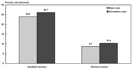
Chart 4 shows the baseline and price indexing simulation poverty rates for disabled-worker and retired-worker beneficiaries. Although the induced changes are comparable for disabled and retired workers in percentage-point terms (2.1 percentage points versus 1.7 percentage points32, the relative changes are much smaller for disabled workers (9 percent versus 20 percent). Thus, the results are somewhat ambiguous, and arguably, the simulations had less of an effect on the prevalence of poverty among disabled workers when compared with retired workers. In any event, the chart clearly indicates that the simulation differences in economic vulnerability are roughly the same for the two groups as they were under the baseline.33 This is so because the simulation poverty rate is dominated by large baseline differences rather than the simulated policy interventions per se, at least for the time horizon of this study.
Poverty rate of disabled and retired workers under baseline and price indexing simulations
| Case | Disabled workers | Retired workers |
|---|---|---|
| Base case | 24.0 | 8.7 |
| Simulation case | 26.1 | 10.4 |
General Distributional Effects
A comprehensive evaluation of simulation results requires an understanding of the underlying mechanisms that produce the distributional outcomes. There are three important factors affecting all OASDI beneficiaries:
- Length of time before OASDI award subject to the new indexing scheme;34
- Availability of SSI; and
- The absolute and relative economic well-being of the family.
Under the assumption of a monotonic increase in real wages (or life expectancy) the first factor is directly related to the design of the two indexing schemes. The simulated OASDI reduction for each individual in the sample is a function of the number of years between the presumed start of the new indexing scheme and the time of claiming benefits. This amount of time—the years of exposure to the new indexing scheme—in combination with the change in the index produces the simulated outcomes. In our observed sample, disabled-worker beneficiaries have shorter durations of benefit receipt than retired-worker beneficiaries (see Table 1). Thus, because the time since the presumed start of the new indexing scheme is divided into the time of exposure to the new scheme and the time of benefit receipt, disabled-worker beneficiaries have more exposure to the new scheme, and consequently, they have larger simulated changes in benefit amounts.
More information about the distribution of benefit duration is given in the Appendix tables. When observed in a cross section, the portion of disabled workers with short durations is relatively large.35 Conversely, the proportion of disabled workers with long duration is relatively small. Short duration in our cross-sectional sample translates into long exposure to the simulated indexing regime. Table A-1 shows that the proportion of disabled-worker beneficiaries with 12–17 years of exposure is 53 percent. In contrast, the average in the general population of beneficiaries (Table A-2) is only 28 percent. These distributional differences reconfirm that the average changes in OASDI benefits corresponding to the simulated indexing approaches are larger for disabled workers than for retired workers.
The importance of length of exposure is further highlighted by the fact that differences in simulated OASDI benefit change levels are not observed for disabled workers when examining the group of relatively new beneficiaries. In contrast to the general population of beneficiaries, the group of new beneficiaries is homogenous in length of exposure to the new indexing scheme. Table 3 shows that the change among beneficiaries who are relatively new beneficiaries (12–17 years of exposure) is 14.6 percent. This is virtually identical to the estimate for disabled workers who are relatively new beneficiaries, 14.7 percent (see Table 4).
| Simulation variable | OASDI benefits a | OASDI plus SSI benefits |
Family income |
|---|---|---|---|
| Years between start of indexing scheme and OASDI award |
|||
| 0–6 | -7.0 (0.056) |
-6.6 (0.061) |
-3.8 (0.053) |
| 7–11 | -10.7 (0.054) |
-10.2 (0.069) |
-5.4 (0.066) |
| 12–17 | -14.6 (0.059) |
-13.8 (0.083) |
-6.3 (0.080) |
| Family income category | |||
| At or below poverty threshold | -9.2 (0.137) |
-6.0 (0.160) |
-5.2 (0.142) |
| Above threshold to 200 percent of poverty threshold |
-9.0 (0.087) |
-8.5 (0.092) |
-6.3 (0.073) |
| Above 200 percent of poverty threshold | -9.9 (0.062) |
-9.8 (0.063) |
-4.0 (0.038) |
| SOURCES: Calculations based on the Survey of Income and Program Participation (SIPP) matched to Social Security administrative records. | |||
| NOTES: The survey reference month is November 1996. The sample is restricted to adults who have SIPP observations that have been successfully matched to the Summary Earnings Record. Sampling weights have been adjusted by the inverse of the matching rate. Standard error estimates assume simple random sampling and are included in parentheses. | |||
| OASDI = Old-Age, Survivors, and Disability Insurance; SSI = Supplemental Security Income. | |||
| a. Values are for the sample reference person if unmarried and for the reference person and spouse combined if married (spouse present). | |||
| Beneficiary characteristic | OASDI benefit a (percent change) |
OASDI plus SSI benefits a (percent change) |
Family income (percent change) |
Poverty rate (percentage- point change) |
Average poverty gap (dollar per month change) |
|---|---|---|---|---|---|
| Years between start of indexing scheme and OASDI award |
|||||
| 0–6 | -3.8 (0.181) |
-3.1 (0.203) |
-1.8 (0.162) |
0.5 (0.552) |
2 (0.729) |
| 7–11 | -9.9 (0.094) |
-8.0 (0.251) |
-4.3 (0.225) |
2.7 (1.104) |
12 (1.542) |
| 12–17 | -14.7 (0.067) |
-12.7 (0.214) |
-5.8 (0.185) |
2.7 (0.648) |
11 (1.109) |
| Family income category | |||||
| At or below poverty threshold | -9.6 (0.325) |
-5.7 (0.377) |
-4.7 (0.331) |
0.0 (0.000) |
33 (2.250) |
| Above threshold to 200 percent of poverty threshold |
-10.7 (0.286) |
-9.4 (0.334) |
-6.2 (0.256) |
7.6 (1.460) |
3 (0.738) |
| Above 200 percent of poverty threshold | -11.1 (0.227) |
-10.6 (0.244) |
-3.2 (0.114) |
0.0 (0.000) |
0 (0.000) |
| Primary insurance amount quartile | |||||
| 1st | -9.8 (0.295) |
-5.0 (0.335) |
-1.9 (0.166) |
0.2 (0.258) |
5 (0.853) |
| 2nd | -10.3 (0.280) |
-10.2 (0.282) |
-5.5 (0.234) |
3.0 (0.906) |
19 (1.666) |
| 3rd | -11.2 (0.402) |
-11.3 (0.401) |
-5.7 (0.363) |
7.6 (2.120) |
9 (2.131) |
| 4th | -11.6 -0.3 |
-11.7 -0.3 |
-5.4 -0.2 |
0.3 -0.3 |
2 -0.9 |
| Age at initial entitlement | |||||
| 18–34 | -7.6 (0.317) |
-5.2 (0.321) |
-2.8 (0.198) |
1.5 (0.667) |
8 (1.206) |
| 35–44 | -10.3 (0.290) |
-8.9 (0.333) |
-4.0 (0.222) |
3.0 (0.928) |
8 (1.286) |
| 45–54 | -12.5 (0.178) |
-11.2 (0.266) |
-5.4 (0.227) |
1.8 (0.707) |
10 (1.407) |
| 55–61 | -15.3 -0.1 |
-14.4 -0.3 |
-6.9 -0.4 |
2.4 -1.3 |
7 -2.2 |
| Education | |||||
| Less than high school | -10.1 (0.272) |
-7.9 (0.328) |
-4.6 (0.236) |
3.2 (0.904) |
12 (1.406) |
| Other | -10.9 (0.191) |
-9.6 (0.221) |
-4.3 (0.149) |
1.6 (0.454) |
7 (0.797) |
| Reported health status | |||||
| Poor | -11.0 (0.250) |
-9.3 (0.302) |
-4.7 (0.216) |
2.2 (0.695) |
9 (1.190) |
| Other | -10.5 (0.201) |
-8.9 (0.233) |
-4.2 (0.156) |
2.1 (0.534) |
8 (0.878) |
| Number of functional impairments b | |||||
| Two or less | -10.7 (0.184) |
-9.1 (0.219) |
-4.3 (0.147) |
1.9 (0.470) |
8 (0.770) |
| Three or more | -10.5 (0.298) |
-9.1 (0.345) |
-4.6 (0.246) |
2.7 (0.899) |
11 (1.539) |
| Primary impairment | |||||
| Mental | -9.6 (0.275) |
-7.3 (0.326) |
-3.8 (0.212) |
3.1 (0.887) |
9 (1.230) |
| Other | -11.2 (0.188) |
-9.9 (0.217) |
-4.7 (0.157) |
1.6 (0.456) |
9 (0.864) |
| Death within 4 years of disability c | |||||
| Yes | -16.1 (0.212) |
-16.1 (0.212) |
-8.0 (0.933) |
5.1 (4.155) |
7 (4.304) |
| Other | -15.1 (0.063) |
-12.9 (0.245) |
-5.7 (0.205) |
1.8 (0.597) |
11 (1.275) |
| Death within 4 years of survey | |||||
| Yes | -11.1 (0.505) |
-10.6 (0.560) |
-5.7 (0.459) |
4.9 (2.120) |
8 (2.441) |
| No | -10.6 (0.165) |
-8.9 (0.195) |
-4.3 (0.131) |
1.9 (0.416) |
9 (0.739) |
| SOURCES: Calculations based on the Survey of Income and Program Participation (SIPP) matched to Social Security administrative records. | |||||
| NOTES: The survey reference month is November 1996. The sample is restricted to adults who have SIPP observations that have been successfully matched to the Summary Earnings Record. Sampling weights have been adjusted by the inverse of the matching rate. Standard error estimates assume simple random sampling and are included in parentheses. | |||||
| OASDI = Old-Age, Survivors, and Disability Insurance; SSI = Supplemental Security Income. | |||||
| a. Values are for the sample reference person if unmarried and for the reference person and spouse combined if married (spouse present). | |||||
| b. Number of difficulties with any activities of daily living (ADL) or instrumental activities of daily living (IADL). | |||||
| c. Subgroup means are limited to the subsample with an estimated duration of 4 years or less at November 1996 reference month. | |||||
The cross-sectional results related to duration of benefit receipt are not expected to apply to other samples, such as a longitudinal sample following a birth cohort. In fact, using a life-cycle perspective, Mermin (2005) has predicted that the timing of benefit claiming would lead to the opposite result: smaller OASDI benefit changes for disabled-worker beneficiaries. Mermin's conclusions are not inconsistent with our findings, however, when the differences in analytical approach (birth cohort versus cross sectional) are removed; the study does focus on outcomes for members of the same birth cohort at ages 62–65 and 80–85. The "disabled" in Mermin's study are either very close to the historical full retirement age or are actually older retired workers (80–85) who are former disability beneficiaries. When we restrict our sample to current retired-worker beneficiaries, we get similar results; previous disabled-worker beneficiaries have smaller simulated changes in OASDI benefits than other retired-worker beneficiaries (see Table 2).
In addition to the length of time subject to the new indexing scheme, other factors that affect the simulated outcomes include the availability of SSI and the effects of total family income.
Table 3 demonstrates each of these effects within the population of OASDI beneficiaries. There is a clear positive relationship between the years subject to the new indexing scheme and the magnitude of percentage changes in average OASDI benefits, OASDI and SSI combined, and family income. It is also notable that within each of the three categories there is a clear pattern indicating the dampening effect of both SSI and other family income.36
The role of the second and third factors can be represented in a unified framework if we look at the three outcome variables as a function of family income relative to the poverty threshold. In Table 3 we create three family income categories representing:
- Those at or below the official poverty threshold;
- Those above the poverty threshold but below twice the threshold; and
- Those above twice the poverty threshold.
Looking at these three categories we can see that the percent reduction in family income is lowest in the third category, second in the first category, and largest in the second category. The data clearly show that the magnitude of OASDI reductions is not responsible for this pattern. SSI plays the largest role for the first category, and virtually no role for the third category. Other income is more important for the second and third categories, with the third category experiencing the larger dampening effect. In summary, the SSI offset is the key mechanism at the lower tail of the income distribution, and other family income is the key mechanism at the higher end of the distribution.
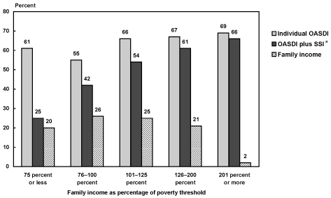
In addition to the dampening effect of SSI and other family income, these same factors also reduce the variability of simulation outcomes. Chart 5 focuses directly on the proportion with relatively large changes (10 percent or larger reductions) in three outcome variables using the group of disabled workers as an example. The results dramatically indicate the dampening role of SSI at the lower tail of the relative income distribution, and the overwhelming buffering role of other family income in the top group.
Percentage of disabled-worker beneficiaries with 10 percent or larger reduction of various outcomes, by family income category
| Reductions of 10 percent or more in— |
75 percent or less |
76–100 percent |
101–125 percent |
126–200 percent |
201 percent or more |
|---|---|---|---|---|---|
| Individual OASDI | 61 | 55 | 66 | 67 | 69 |
| OASDI plus SSI a | 25 | 42 | 54 | 61 | 66 |
| Family income | 20 | 26 | 25 | 21 | 2 |
The evidence in this section all refers to the price indexing simulation. However, the mechanisms described above apply to the life expectancy simulation as well. Because the relative outcomes are very similar for both sets of simulations, we present only the results for price indexing.
Disabled-Worker Beneficiaries
In this section we provide a more detailed analysis of the simulated effects on disabled beneficiaries. Several concerns motivate our focus here. First, we would like to confirm our expectation that the same mechanisms that explained the overall results for all OASDI beneficiaries are detectable among disabled-worker beneficiaries as well. Second, we have seen that the disabled as a group had a high level of economic vulnerability under the baseline. Even though the differences in the overall effects of the indexing approaches between disabled and retired workers were relatively small, it is possible that the indexing approaches have particularly unfavorable effects on some subgroups of disabled workers. We examine the subgroups identified as economically vulnerable above including those in the lowest PIA quartile, with less than a high school education, with an early onset of disability, or a primary mental impairment.
Table 4 shows that the same underlying mechanisms are at work for disabled workers as for OASDI beneficiaries in general. For "years between start of indexing scheme and OASDI award," there is a wide dispersion of outcomes across categories. As before, those with the longest exposure to the new indexing scheme experience the largest changes. Also, SSI has a visible impact on outcomes for those below the poverty thresholds whereas other family income has a noticeable impact for those above twice the poverty thresholds. In addition to the subgroup in poverty, the role of SSI is also notable for the four other economically vulnerable subgroups. When SSI is considered together with OASDI, the changes are relatively small for all these subgroups. For two of the subgroups, those without a high school education and those with a primary mental diagnosis, we compare the vulnerable subgroups with the group of all other disabled workers. By comparison, we use the adjacent subgroup for those with an early onset of disability (the next earliest entitlement age category) and those in the lowest PIA quartile (the second PIA quartile). For all of these subgroups, the estimated change in total benefits is smaller than for the comparison subgroup and these comparisons are all statistically significant.
These differences do not imply that vulnerability would not be a concern for these subgroups under the alternative indexing approaches. We use the subgroup of disabled beneficiaries in poverty as an illustration. For this subgroup, the change in total benefits is -5.7 percent compared with -9.4 percent for the subgroup between the poverty level and twice the poverty level.37 In the base case, these two subgroups had average benefits of $532 and $737 respectively (Table A-1), a difference of $205. These amounts changed to $502 and $668 respectively under the price indexing approach, a difference of $166. Thus, the percentage changes translate into narrowing the difference in average total benefits between subgroups by $39. This is less than 20 percent of the original difference. Similar comparisons hold for the four economically vulnerable subgroups.38 At least for the analysis period of this study, differences in simulated average total benefits among disabled-worker beneficiaries are dominated by baseline differences rather than the effects of the alternative indexing approaches.
When we examine other aspects of vulnerability that are not associated with poverty, such as severity of impairment and expected mortality, we generally do not find meaningful differences. The one exception is for mortality within 4 years of the onset of disability and the differences are significant only for the outcome of total benefits. For this outcome, the subgroup with high mortality has a larger simulated benefit change.
Conclusions and Implications
In this study, we found similar impacts of changing the indexing scheme on disabled-worker beneficiaries and retired-worker beneficiaries. While the change in OASDI benefits is larger for disabled workers, the counterbalancing effect of SSI is also larger. This is partly due to higher rates of SSI eligibility among disabled workers relative to retired workers, and partly due to higher rates of SSI participation. As a result, the overall differences between disabled- and retired-worker beneficiaries are small and not statistically significant. Since the prevalence of poverty is relatively high among the disabled under the status quo, the relative economic vulnerability of the disabled would change only slightly.
Moreover, disaggregated estimates indicate that economically vulnerable groups of disabled-worker beneficiaries would be less affected by the alternative indexing approaches than disabled workers in general. Thus, the alternative indexing approaches would lead to a narrowing of the distribution of well-being within the group of disabled-worker beneficiaries. However, the magnitudes of the estimated changes are small compared with the differences in well-being in the status quo.
These results are due to three general distributional effects that affect outcomes on an individual level, including 1) the number of years that a person is subject to the new indexing approach, 2) the offsetting effect of the SSI program, and 3) the diluting effect of other family income. Thus, changes in distributional outcomes are due to differences within and between groups in the timing of entitlement to benefits, participation in the SSI program and, naturally, differences in family economic well-being.
We conclude by discussing four study features that affect the interpretation of our results. One concern is whether the study results are generalizable, that is, whether they are robust to the choice of analytical perspective. A second issue is whether results based on the current stock of beneficiaries are applicable to future beneficiary populations, especially given secular changes in the age and diagnostic mix of awardees. A third concern is the effect of the analysis period on the distributional analysis. What are the potential effects of using a shorter or longer time horizon for the analysis? Fourth, we discuss how the consideration of behavioral effects might alter the results.
Generalizability
We have found that although the indexing schemes were designed to result in proportional changes in benefits for new awardees in a given year, the effects of these changes on the family income of the beneficiaries would vary across individuals because of differences in the timing of benefit claiming, the offsetting effect of SSI, and the diluting effect of other sources of family income. Although the observed differences that are associated with the timing of benefit claiming are sensitive to the analytic perspective (such as cross section, birth cohort, or new awardee cohort comparisons), the roles of SSI and other sources of family income in dampening the effects of indexing changes seem fairly robust to a variety of factors and assumptions. The following paragraphs provide a brief summary of our assessment of the generalizability of our key results.
There will be an SSI offset effect as long as new OASDI awardees are financially eligible for SSI or would become financially eligible as a result of OASDI benefit reductions. For example, whether we use a cross-sectional or another analytical perspective, based on the current income distribution, there will always be beneficiaries for whom SSI will offset some of the OASDI reductions. Because disabled-worker beneficiaries are more likely than retired-worker beneficiaries to be in the lower tail of the income distribution, SSI will tend to have a relatively large dampening effect for disabled workers. Further, this effect will be magnified by higher SSI participation rates among disabled workers than retired workers. While the directions of these effects seem robust to analytical choices made by the researcher, the magnitudes might depend heavily on assumptions made about future trends. For example, the results of a study that estimates the effects of the reforms on a young birth cohort into the future would depend on the assumptions made about future trends in real wage growth and income inequality. By contrast, our study uses historical trends.
Similarly, the effects of other sources of family income should be robust to choice of analytical perspective, although other studies may make different assumptions about family wage growth and distribution. In our study, we have found that this dampening effect is important for both disabled and retired workers. Based on the observed distribution of income, disabled-worker and retired-worker beneficiaries have similar levels of family income on average. However, the distribution of family income is considerably more disperse for disabled workers. Studies using other analytical perspectives would need to consider these differences in income distribution.
Applicability to Future Beneficiary Stocks
The generalizability of our results to more recent or future target populations is a natural concern given that the characteristics of the disability caseload have changed substantially over the past couple of decades. For example, a secular shift to younger new awardees and toward mental impairments is clearly observable. Also, the aging of the baby boom generation will affect the trend in the age distribution of awardees.
For these factors to have a substantial effect on the generalizability of our results, two conditions must hold. First, there must be substantial change in at least one of the compositional variables measuring the mix of the target population (for example in age distribution), and, second, there must be an association between this variable and the simulation outcome of interest. This article has provided new evidence on the second condition. For example, younger age at onset of disability is associated with relatively low reductions in benefits (Table 4). Also, estimated changes for those with a primary mental impairment are smaller than for other types of impairments on average. Thus, we can surmise that a shift toward younger new DI awardees and toward mental diagnoses might result in smaller average benefit changes for a future caseload than would be the case without changes in the future diagnostic mix. As a result, our results might overestimate the magnitude of changes for the disabled attributable to the change in indexing scheme.
Relevance of Analysis Period to Distributional Results
The empirical estimates presented in this study are all conditional on the assumption that the shift in the indexing approach occurred 17 years before the reference month. This implies that the length of time between the change in indexing and the OASDI award can vary between 0 and 17 years for an individual. In theory, one can reduce (let us say to 10 years) or increase (to 20, 30, or 40 years) the length of the time from the start of the alternative indexing approach to the reference period of interest.
As long as one is maintaining the assumption of real wage (or life expectancy) increases, the nature of the indexing approaches is such that the magnitude of changes in OASDI benefits should increase as a positive function of the length of time elapsing after the introduction of the new indexing approach. The magnitudes will generally increase with an increasing time period into the indefinite future.
This relationship needs to be considered in any comparisons with studies that employ a different time horizon. Further, can we make inferences about the effect of different time horizons on distributional outcomes? For example, what can we say about the effects of SSI and other family income? Under reasonable assumptions, we can make plausible inferences about both. Note that under current law, the SSI federal benefit rate is indexed to inflation.39 Because the magnitudes of OASDI benefit changes are expected to increase as a positive function of the time horizon, an increasing proportion of OASDI beneficiaries will meet the SSI financial eligibility test. It follows that SSI will offset the changes in OASDI benefits for an increasing number of beneficiaries. Likewise, the buffering role of other family income is also expected to increase as we increase the time horizon of the analysis. Finally, as we extend the time horizon of the implementation of the alternative indexing approach, the effects of the change in indexing should become an increasingly important influence on well-being relative to the influence of the status quo.
Behavioral Responses
Our findings reflect the "direct effect" (see Bound and others 2002) of the indexing approaches and are predicated on the simplifying assumption of no behavioral effects. Are the empirical results robust to the assumption of no behavioral effects? To answer this question empirically requires a model capable of capturing "indirect (behavioral) effects." Behavioral changes in program participation may be relevant as well as behavioral changes in labor markets, financial markets, and private disability insurance markets.
Changes in program participation may be particularly relevant in this case because participation in the DI program may be more or less responsive to the change in indexing approach than participation in the OASI program. For example, disabled people face substantial opportunity costs as a result of the disability determination process, but may be more constrained in their choices as a result of their disabling conditions than people contemplating early retirement.
Since the simulated changes in total benefits are comparable for disabled- and retired-worker beneficiaries, whether disabled-worker beneficiaries are more or less affected in the aggregate will mainly be a function of the relative elasticities for the two groups. For disability, reduced benefit levels are expected to result in lower lifetime participation in the DI program. For retirement, benefit levels are expected to primarily affect the timing of retirement, particularly early retirement.
Perhaps a firmer expectation of the importance of "indirect effects" can be made by considering the degree of economic vulnerability of the disabled group. Disabled workers are more likely to be in poverty and, further, the "direct effects" (for OASDI and SSI combined) are lower for those in poverty. Thus, we surmise that unless participation in the DI program is much more responsive to changes in the bundle of expected benefits, the qualitative conclusions will be robust to the consideration of behavioral effects.
Appendix
This appendix gives information about the baseline values of the analysis variables. Table A-1 gives the values for disabled-worker beneficiaries and Table A-2 gives the values for the entire sample of OASDI beneficiaries as background for the section on general distributional effects.
| Beneficiary characteristic at baseline | Distribution at baseline (percent) |
Subgroup mean at baseline | ||||
|---|---|---|---|---|---|---|
| Individual OASDI benefits a (dollars) |
Unit OASDI benefits b (dollars) |
Unit OASDI plus SSI benefits b (dollars) |
Family income (dollars) |
Poverty rate (percent) |
||
| Primary insurance amount quartile c | ||||||
| 1st | 31 | 365 (5) |
407 (11) |
477 (10) |
2,193 (195) |
43.8 (2.6) |
| 2nd | 30 | 593 (4) |
635 (10) |
639 (10) |
2,108 (94) |
30.3 (2.4) |
| 3rd | 14 | 783 (3) |
836 (15) |
836 (15) |
2,774 (182) |
5.5 (1.8) |
| 4th | 25 | 1,054 (7) |
1,111 (13) |
1,111 (13) |
3,711 (262) |
1.6 (0.8) |
| Family income category | ||||||
| At or below poverty threshold | 24 | 466 (9) |
474 (10) |
532 (8) |
690 (20) |
100.0 (0.0) |
| Above threshold to 200 percent of poverty threshold |
28 | 667 (14) |
719 (16) |
737 (15) |
1,421 (35) |
0.0 (0.0) |
| Above 200 percent of poverty threshold | 48 | 758 (13) |
822 (15) |
831 (15) |
4,279 (179) |
0.0 (0.0) |
| Years between start of stimulated policy change and OASDI award |
||||||
| 0–6 | 15 | 593 (18) |
614 (20) |
640 (19) |
2,316 (138) |
26.2 (3.4) |
| 7–11 | 22 | 643 (17) |
691 (22) |
720 (20) |
2,337 (121) |
29.6 (2.8) |
| 12–17 | 53 | 697 (12) |
750 (14) |
770 (13) |
2,916 (168) |
20.0 (1.6) |
| Award before policy change | 9 | 633 (29) |
684 (33) |
705 (31) |
2,151 (201) |
29.4 (4.5) |
| Age at initial entitlement d | ||||||
| 18–34 | 30 | 543 (13) |
564 (15) |
605 (14) |
2,329 (118) |
35.1 (2.6) |
| 35–44 | 30 | 679 (15) |
703 (16) |
724 (15) |
2,784 (256) |
21.0 (2.2) |
| 45–54 | 29 | 723 (15) |
790 (18) |
803 (17) |
2,601 (146) |
20.6 (2.2) |
| 55–61 | 11 | 793 (25) |
899 (34) |
909 (33) |
3,075 (252) |
10.6 (2.7) |
| Education | ||||||
| Less than high school | 32 | 601 (13) |
657 (17) |
693 (15) |
1,982 (177) |
34.5 (2.5) |
| Other | 68 | 692 (10) |
734 (12) |
752 (11) |
2,925 (116) |
19.0 (1.4) |
| Reported health status | ||||||
| Poor | 37 | 671 (12) |
716 (15) |
742 (13) |
2,271 (97) |
25.4 (2.1) |
| Other | 63 | 658 (11) |
706 (13) |
728 (12) |
2,832 (145) |
23.1 (1.6) |
| Number of functional impairments | ||||||
| Two or less | 71 | 663 (10) |
707 (12) |
730 (11) |
2,610 (108) |
23.2 (1.5) |
| Three or more | 29 | 663 (15) |
717 (18) |
740 (17) |
2,660 (210) |
25.8 (2.4) |
| Primary impairment | ||||||
| Mental | 33 | 572 (14) |
589 (15) |
629 (13) |
2,191 (106) |
30.4 (2.4) |
| Other | 67 | 708 (10) |
770 (12) |
785 (12) |
2,842 (136) |
20.7 (1.5) |
| Death within 4 years of onset e | ||||||
| Yes | 6 | 761 (51) |
887 (64) |
887 (64) |
2,504 (291) |
3.9 (3.7) |
| Other | 94 | 695 (13) |
743 (15) |
764 (14) |
3,035 (202) |
20.1 (1.8) |
| Death within 4 years of survey | ||||||
| Yes | 9 | 744 (26) |
815 (32) |
824 (31) |
2,312 (170) |
15.5 (3.6) |
| No | 91 | 655 (9) |
700 (10) |
724 (10) |
2,655 (106) |
24.8 (1.3) |
| SOURCES: Calculations based on the Survey of Income and Program Participation (SIPP) matched to Social Security administrative records. | ||||||
| NOTES: The survey reference month is November 1996. The sample is restricted to adults who have SIPP observations that have been successfully matched to the Summary Earnings Record. Sampling weights have been adjusted by the inverse of the matching rate. Standard error estimates assume simple random sampling and are included in parentheses. | ||||||
| OASDI = Old-Age, Survivors, and Disability Insurance; SSI = Supplemental Security Income. | ||||||
| a. Values are for the sample reference person. | ||||||
| b. Values are for the sample reference person if unmarried and for the reference person and spouse combined if married (spouse present). | ||||||
| c. Quartile of primary insurance amounts among all beneficiaries. | ||||||
| d. An estimated 0.4 percent of the sample was aged 62–64 at the time of initial entitlement. Subgroup means are not shown for this subcategory. | ||||||
| e. Subgroup means are limited to the subsample with an estimated duration of 4 years or less at November 1996 reference month. | ||||||
| Beneficiary characteristic at baseline | Distribution at baseline (percent) |
Subgroup mean at baseline | ||||
|---|---|---|---|---|---|---|
| Individual OASDI benefits a (dollars) |
Unit OASDI benefits b (dollars) |
Unit OASDI plus SSI benefits b (dollars) |
Family income (dollars) |
Poverty rate (percent) |
||
| Primary insurance amount quartile | ||||||
| 1st | 25 | 335 (2) |
545 (6) |
584 (6) |
2,181 (51) |
29.6 (0.9) |
| 2nd | 25 | 605 (1) |
814 (6) |
815 (6) |
2,208 (41) |
15.1 (0.7) |
| 3rd | 25 | 794 (1) |
1,142 (8) |
1,142 (8) |
2,655 (43) |
1.0 (0.2) |
| 4th | 25 | 989 (3) |
1,395 (9) |
1,395 (9) |
3,479 (63) |
0.4 (0.1) |
| Family income category | ||||||
| At or below poverty threshold | 11 | 422 (4) |
449 (5) |
502 (4) |
612 (8) |
100.0 (0.0) |
| Above threshold to 200 percent of poverty threshold |
27 | 641 (4) |
791 (6) |
800 (5) |
1,205 (9) |
0.0 (0.0) |
| Above 200 percent of poverty threshold | 62 | 736 (3) |
1,136 (6) |
1,138 (6) |
3,606 (37) |
0.0 (0.0) |
| Years between start of stimulated policy change and OASDI award |
||||||
| 0–6 | 26 | 680 (5) |
968 (9) |
977 (9) |
3,082 (58) |
10.4 (0.6) |
| 7–11 | 24 | 700 (5) |
1,073 (10) |
1,082 (10) |
2,771 (50) |
9.3 (0.6) |
| 12–17 | 28 | 666 (5) |
967 (9) |
976 (9) |
2,489 (48) |
10.5 (0.6) |
| Award before policy change | 21 | 651 (5) |
840 (9) |
852 (8) |
2,029 (41) |
15.9 (0.8) |
| Education | ||||||
| Less than high school | 34 | 613 (4) |
844 (7) |
864 (7) |
2,004 (35) |
19.6 (0.6) |
| Other | 66 | 707 (3) |
1,030 (6) |
1,034 (6) |
2,947 (34) |
7.0 (0.3) |
| Reported health status | ||||||
| Poor | 15 | 624 (6) |
839 (11) |
860 (10) |
2,145 (54) |
20.0 (1.0) |
| Other | 85 | 684 (3) |
988 (5) |
995 (5) |
2,707 (29) |
9.8 (0.3) |
| Number of functional impairments | ||||||
| Two or less | 84 | 686 (3) |
997 (5) |
1,004 (5) |
2,702 (27) |
9.7 (0.3) |
| Three or more | 16 | 619 (6) |
802 (10) |
823 (10) |
2,207 (72) |
20.2 (1.0) |
| Death within 4 years of survey | ||||||
| Yes | 13 | 666 (7) |
922 (12) |
931 (12) |
2,379 (66) |
12.7 (0.9) |
| No | 87 | 676 (3) |
972 (5) |
982 (5) |
2,660 (28) |
11.1 (0.3) |
| SOURCES: Calculations based on the Survey of Income and Program Participation (SIPP) matched to Social Security administrative records. | ||||||
| NOTES: The survey reference month is November 1996. The sample is restricted to adults who have SIPP observations that have been successfully matched to the Summary Earnings Record. Sampling weights have been adjusted by the inverse of the matching rate. Standard error estimates assume simple random sampling and are included in parentheses. | ||||||
| OASDI = Old-Age, Survivors, and Disability Insurance; SSI = Supplemental Security Income. | ||||||
| a. Values are for the sample reference person. | ||||||
| b. Values are for the sample reference person if unmarried and for the reference person and spouse combined if married (spouse present). | ||||||
Distribution of simulated changes in benefits under life expectancy indexing for disabled- and retired-worker beneficiaries
Text description for Chart A-1.
Distribution of simulated changes in benefits under life expectancy indexing for disabled- and retired-worker beneficiaries
This chart shows four separate panels of bar charts. The first two panels show data for OASDI benefits, one panel for disabled-worker beneficiaries and one panel for retired-worker beneficiaries. The final two panels show data for OASDI plus SSI benefits, one panel for disabled-worker beneficiaries and one panel for retired-worker beneficiaries.
In all panels, the horizontal axis shows the percent change in benefits under life expectancy indexing and the vertical axis shows the percentage of beneficiaries. Vertical bars in each panel indicate the percentage of beneficiaries with benefits changing by certain percentages.
In the panel for disabled-worker OASDI beneficiaries, the bars reach the following approximate coordinates: 18 percent of beneficiaries at minus 7.8 percent; 20 percent of beneficiaries at minus 7.0 percent; 16 percent of beneficiaries at minus 6.2 percent; six percent of beneficiaries at minus 5.3 percent; 10 percent of beneficiaries at minus 4.5 percent; six percent of beneficiaries each at minus 3.7 percent and minus 2.9 percent; two percent of beneficiaries at minus 2.1 percent; four percent of beneficiaries at minus 1.2 percent; and 11 percent of beneficiaries at minus 0.4 percent.
In the panel for retired-worker OASDI beneficiaries, the bars reach the following approximate coordinates: 15 percent of beneficiaries at minus 7.8 percent; nine percent of beneficiaries each at minus 7.0 percent and minus 6.2 percent; six percent of beneficiaries at minus 5.4 percent; 25 percent of beneficiaries at minus 4.5 percent; eight percent of beneficiaries at minus 3.7 percent; six percent of beneficiaries each at minus 2.9 percent and minus 2.1 percent; five percent of beneficiaries at minus 1.2 percent; and 12 percent of beneficiaries at minus 0.4 percent.
In the panel for disabled-worker OASDI plus SSI beneficiaries, the bars reach the following approximate coordinates: 16 percent of beneficiaries at minus 7.8 percent; 17 percent of beneficiaries at minus 7.0 percent; 13 percent of beneficiaries at minus 6.1 percent; five percent of beneficiaries at minus 5.3 percent; eight percent of beneficiaries at minus 4.5 percent; five percent of beneficiaries each at minus 3.7 percent and minus 2.9 percent; two percent of beneficiaries at minus 2.0 percent; three percent of beneficiaries at minus 1.2 percent; and 25 percent of beneficiaries at minus 0.4 percent.
In the panel for retired-worker OASDI plus SSI beneficiaries, the bars reach the following approximate coordinates: 14 percent of beneficiaries at minus 7.8 percent; eight percent of beneficiaries at minus 7.0 percent; nine percent of beneficiaries at minus 6.2 percent; five percent of beneficiaries at minus 5.4 percent; 24 percent of beneficiaries at minus 4.5 percent; eight percent of beneficiaries at minus 3.7 percent; six percent of beneficiaries at minus 2.9 percent; five percent of beneficiaries each at minus 2.1 percent and minus 1.2 percent; and 15 percent of beneficiaries at minus 0.4 percent.
In addition to the bars, a line labeled Kernal density function appears on all panels. The line roughly follows the tops of the vertical bars.
Notes
1. In addition to indexing provisions, the CSSS reform models have other important elements. For example, the minimum benefit provisions and changes in the benefit formulas for widow(er)s would affect the population that is eligible for SSI. Other plans that have been proposed also include indexing provisions. In this article we are focusing on indexing and do not attempt to model other provisions of the CSSS reform models or other approaches.
2. Munnell and Soto (2005) also describe the transition properties of some of these variants of the alternative methods of implementation. On the revenue side, the General Accountability Office (2006) explores different effects of wage and price indexing on system revenues through the mechanism of the taxable maximum.
3. See Munnell and Soto (2005) for one justification.
4. The historical full retirement age, 65, is used.
5. See CSSS (2001), p. 132.
6. See CSSS (2001) p. 132.
7. See CSSS (2001) p. 149.
8. Government Accountability Office (2007) is another example of analysis from a birth cohort perspective.
9. The estimates ignore the effect that the family maximum may have on the simulated benefit changes.
10. For retired-worker beneficiaries, we assume that entitlement is at age 62 with the corresponding reduction in benefits.
11. The calculated benefit amounts correspond closely to the amounts given in the administrative records. For instance, the average calculated benefit amount is 100.0 percent and 97.8 percent of the average administrative amount for disabled and retired workers, respectively.
12. For comparison, we also estimated the impact using the actual trends in wages and prices over the 1977 to 1994 period (accounting for the 2-year lags). Although wages are shown to grow faster than prices over the long term, there was a reversal of this trend during the high-inflation period of the late 1970s. The net result is that there is almost no change in the relative position of wages and prices during our analysis period. Simulations based on the observable trend during this period show an overall change in OASDI benefits of -0.4 percent and 0.3 percent for disabled and retired workers respectively, magnitudes that are not statistically significantly different from zero. In the case of retired workers, the simulation results do not even have the sign expected by proponents of the indexing changes (negative).
13. We have chosen the starting point for the alternative indexing approaches in order to isolate the effects of a single policy change: the shift from wage indexing to price indexing (or life expectancy indexing). Given this starting date, beneficiaries initially entitled to benefits before 1979 are unaffected by the alternative indexing approaches. Note that for observations with an initial entitlement after the start of the current regime of indexing, all earnings are indexed in order to calculate the AIME, including earnings before 1979.
This starting date may introduce an upward (more negative) bias in the estimated changes for beneficiaries whose entitlement was near the start of the current regime of indexing. During this period, beneficiaries were given the higher of the benefit calculated under the old and new formulas. Consequently, hypothetical changes could possibly have been counteracted by this provision if the old formula produced a higher benefit than the simulation (hypothetical) formula.
14. As with OASDI, we do not estimate changes in SSI benefits for family members other than the self and spouse. Also, we consider only federal SSI benefits and not state SSI supplements.
15. We assume that concurrent beneficiaries under the baseline also participate in SSI under the alternative indexing approaches. This is a reasonable assumption because this set of beneficiaries is observed to participate in the SSI program at a lower SSI benefit amount than might be available to them under the alternative indexing approaches. Note, however, that there are other OASDI beneficiaries who are eligible for SSI and choose not to participate or are ineligible but become eligible as a result of reduced income from OASDI. We conservatively assume that members of both of these groups will continue not to participate in SSI under the alternative indexing approaches.
16. The standard errors used in statistical tests need to be adjusted in order to account for the complex sample design of the SIPP. We give unadjusted standard errors in the tables; however, we use an approximate adjustment for statistical tests. The U.S. Census Bureau (2001) gives design effects (adjustment factors) accounting for the effect of the complex sample design on the variances of various survey items. Because the estimated design effect exceeds four only for one item (metro status), and is much smaller for other survey items, we adopt a design effect of four for the variances. This implies true standard errors that are twice as large as the unadjusted standard errors. Assuming a design effect of four provides conservative tests of population differences. All statistical tests are performed at the 5 percent level of significance.
17. We do not employ the group that we label "Other Beneficiaries" as a comparison group because it is heterogeneous and has markedly different demographic characteristics than the other groups. Primarily, the group differs in that it has mostly women and has a lower percentage of people that are married or have finished high school. These differences are statistically significant.
18. Interestingly, the potential (calculated) average benefit of nonbeneficiaries (assuming a hypothetical entitlement date of the reference month) is $667, a point estimate very close to the average benefit for the disabled.
19. Both of these averages refer to the average for the reference person. In general, all unit averages are based on the unit variable associated with the sample reference person because the unit of analysis is the individual throughout the study.
20. Kernel density estimators provide a visual representation of the distribution of observations similar to bar charts of frequency distributions. In contrast to bar charts, they provide a smooth curve.
21. A bimodal distribution is not observed when benefits are measured on an individual basis (not shown).
22. Authors' calculations.
23. Authors' calculations.
24. While the high mortality groups actually have lower poverty rates than the comparison groups, the differences are not statistically significant. Contributing factors include the strict statistical tests we employ and the sample size of the group with an onset of disability within 4 years of the survey. Thus the conclusion of no evidence of a positive relationship with economic vulnerability is supported by the data.
25. Heterogeneity within the group of retired workers modifies the main result. Among retired workers, a statistically significant difference is evident between the average benefits of retired workers who were never disabled workers and the average benefits of retired workers who had converted from the DI program.
26. Of the distributional effects considered below, the only one that can vary across spouses is the length of time the person is subject to the alternative indexing approach (inversely related to duration of benefit receipt).
27. The differences between the individual and unit OASDI benefit change statistics are generally small and not statistically significant. Further, meaningful differences are also not observed between the distributions of individual and unit OASDI benefits for sample beneficiaries. In general, this means that differences in statistics between "individual OASDI benefits" and "unit OASDI plus SSI benefits" are exclusively attributable to the inclusion of SSI benefits rather than to the shift from the individual to the unit OASDI benefit. Thus, we include unit changes in subsequent tables and drop individual-only benefit changes.
28. The comparison is on a unit basis.
29. The SSI income eligibility rules allow for the exclusion of up to $20 from any source in the benefit calculation. Thus a concurrent individual or couple beneficiary with $20 of OASDI benefits and no income from other sources under the baseline would experience no increase in the SSI benefit with any simulated reduction in the OASDI benefit. Similarly, an individual or couple with $30 of OASDI benefits would have a 100 percent potential offset for the first $10 reduction in OASDI benefits and no offset for additional reductions. In general, the SSI offset would be reduced from the 100 percent rate only if the OASDI change results in a benefit less than $20 and there is no or only very little countable income from other sources.
30. We do not present the distributions for family income changes in this article; however, we note that the distribution becomes unimodal for both groups (with a peak at the smallest change category). Also, although the proportion with essentially no change in family income is much higher for disabled workers, the proportion with relatively large changes (15 percent or more) continues to appear somewhat larger for the disabled. Thus, the dampening effects of SSI and other family income might not entirely eliminate the greater variability for disabled workers.
31. More formally, if I(B) is the baseline value of a distributional indicator, and I(S) is the corresponding simulation value, then the first perspective focuses on ∆ I = I(S) – I(B). The second perspective focuses on I(S), which equals I(B) + ∆ I.
32. This difference is not statistically significant.
33. Of course, economic vulnerability increases for both groups relative to the baseline as a result of the simulated policy changes that were designed to reduce the growth of benefits across the board.
34. For those observed in the cross section, there is an exact mathematical relationship between duration and our measure of the length of time between the start of the new indexing scheme and award. Duration equals 17 years minus the length of time before OASDI award subject to the new indexing scheme. For members of the same birth cohort there is a similar relationship between age at entry and our length measure. However, people with identical age at entry in the cross section may belong to different birth cohorts and therefore the relationship between age at entry and our length measure is more indirect.
35. Our cross-section estimates of duration reflect right-censoring at the survey reference month. Therefore they are not indicative of lifetime duration on DI. Indeed, Rupp and Scott (1998) provide cohort-based estimates of duration on disability before age 62 that are clearly higher. Considering the fact that many disabled people survive until age 62 and even well after the full retirement age, our cross-sectional estimate of duration would be substantially biased in a downward direction if one mistakenly took it as a proxy for lifetime duration.
36. The starting values for the variables shown in Table 3 are shown in Table A-2.
37. This difference is statistically significant.
38. These differences can be calculated from the figures given in Table 4 and Table A-1.
39. Currently SSI is not a "fully indexed" program because program parameters such as the general income exclusion and the thresholds applied to the resource test are not automatically adjusted for inflation.
References
Bell, Felicitie C., and Michael L Miller. 2002. Life tables for the United States Social Security area 1900–2100. Actuarial Study No. 116, Baltimore, Maryland: Social Security Administration.
Biggs, Andrew G., Jeffery R. Brown, and Glenn Springstead. 2005. Alternative methods of price indexing Social Security: Implications for benefits and system financing, National Tax Journal LVIII(3): 483–504.
Bound, John., Julie B. Cullen, Austin Nichols, and Lucy Schmidt. 2002. The welfare implications of increasing Disability Insurance benefit generosity. NBER Working Paper Number 9155, Cambridge, Massachusetts: National Bureau of Economic Research.
Chaplain, Chris, and Alice H. Wade. 2005. Estimated OASDI long-range financial effects of several provisions requested by the Social Security Advisory Board. Memorandum to Stephen C. Goss, Chief Actuary, Social Security Administration, Office of the Chief Actuary (February 7).
Davies, Paul S., Minh Huynh, Chad Newcomb, Paul K. O'Leary, Kalman Rupp, and Jim Sears. 2001/2002. Modeling SSI financial eligibility and simulating the effect of policy options. Social Security Bulletin 64(2): 16–45.
Government Accountability Office. 2006. Social Security reform: Implications of different indexing choices. Report to Congressional Addressees, GAO-06-804 (September).
———. 2007. Social Security Reform: Issues for Disability and Dependent Benefits. Report to Congressional Requesters, GAO-08-26 (October).
Goss, Stephen C., and Alice H. Wade. 2002. Memorandum to Daniel Patrick Moynihan and Richard Parsons, Co-Chairs, President's Commission to Strengthen Social Security.
———. 2006. Estimated Financial Effects of a Proposal to Restore Sustainable Solvency for the Social Security Program. Memorandum to Senator Robert Bennett, Vice Chairman, Joint Economic Committee of Congress (March 16). http://www.ssa.gov/OACT/solvency/index.html.
Huynh, Minh, Kalman Rupp, and James Sears. 2002. The assessment of Survey of Income and Program Participation (SIPP) benefit data using longitudinal administrative records. SIPP Working Paper No. 238, Washington, DC: U.S. Census Bureau.
Mermin, Gordon B.T. 2005. Distributional effects of reforming Social Security through benefit reductions. The Urban Institute, Publication ID #411260 (December).
Munnell, Alicia H., and Mauricio Soto. 2005. What does price indexing mean for Social Security benefits? Just the Facts on Retirement Issues, Number 14, Center for Retirement Research at Boston College (January).
President's Commission to Strengthen Social Security. 2001. Strengthening Social Security and creating financial wealth for all Americans: Report of the president's commission. Available at http://www.ssa.gov/history/reports/pcsss/reports.html (December).
Rupp, Kalman, and Charles Scott. 1998. Determinants of duration on the disability rolls and program trends. In Growth in disability benefits: Explanations and policy implications, ed. K. Rupp and D. Stapleton, Kalamazoo, MI: The Upjohn Institute.
U.S. Census Bureau. 2001. Source and accuracy statement for the 1996 public-use files from the Survey of Income and Program Participation, Washington, DC: U.S. Census Bureau.